Authors
Nairit Barkataki*, Banty Tiru# and Utpal Sarma*
* Dept of Instrumentation & USIC, Gauhati University, Guwahati, India
# Dept of Physics, Gauhati University, Guwahati, India
Note:
This article was published in the Journal of Applied Geophysics You may cite the article using the following bibliographic data:
© 2022 Elsevier B.V.
Contents
1. Introduction
1.1. Literature Review
1.2. Aim of Present Work
2. GPR Data
3. GPR Principle
4. Convolution Neural Networks
5. Proposed CNN Architecture
5.1. Feature Extraction
5.1.1. Sobel Operator
5.1.2. Laplacian Operator
5.1.3. Canny Operator
5.2. Training of CNN model
5.2.1. Convolution Layer
5.2.2. Pooling Layer
5.2.3. Fully Connected Layer
5.2.4. Loss Function
5.2.5. Optimization
5.2.6. Evaluation Metrics
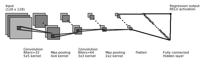
5.3. Final Architecture
6. Results and Discussion
6.1. Testing on noisy data
6.2. Testing on non-metallic buried objects
6.3. Testing on multiple buried objects
7. Conclusion
8. Acknowledgements
9. Data Availability
In recent years, a variety of methods have been proposed by researchers for the interpretation of GPR data. [1] successfully applied the Histograms of Oriented Gradients (HOG) feature extraction technique to landmine detection in GPR data to detect landmines and proposed that other image processing techniques may also be applied for detection of targets in GPR data. A hyperbola fitting technique was used by [2] to estimate the radius of buried pipes and cables. [3] used Fourier Transform and Principal Component Analysis to detect landmines in various burial conditions.
Considerable research has been done in the detection of hyperbolic features and determination of regions of interest in GPR images for further interpretation of various parameters. Different strategies have been used on the topic of hyperbola detection. Fitting algorithms like Radon ([4]), wavelet ([5]) and Hough ([6][7]) have been used for feature extraction in GPR images. Other feature extractors like Sobel operators ([8]) and Canny operators ([9][10]) are also used as a pre-processing step. Statistical approaches like least square ([6]), fuzzy shell clustering ([11]), moment of inertia optimization ([12]) etc., have also been used to extract hyperbolic features. These methods usually involve multi-stage techniques. Initially, a region of interest is determined and then a hyperbola fitting algorithm is applied to it. All these methods are computationally slow but perform well from the point of view of accuracy and sensitivity.
[13] proposed a multi-stage technique which could recognise and fit hyperbolae in real time. They adapted OpenCV library to localise reflection hyperbolas in GPR B-Scans. The developed algorithm showed promising results when applied on using realistic data. They used Canny operator for edge detection and Hough transform for hyperbola fitting. Later, [14] working on a similar problem, proposed a novel technique for real-time hyperbola recognition by using a neural network classification algorithm. They used synthetic input images of size 100 $\times$ 100 pixels. Due to the fast computation speed, both methods proposed by [13] and [14] are suitable for real-time applications.
However, studies by [15] have shown that under certain conditions, Common Midpoint (CMP) method appeared to be a more accurate way to determine GPR subsurface velocity than hyperbola fitting. [16] applied CMP method when estimating the thickness of asphalt.
Machine learning algorithms can be used for meaningful interpretation of GPR data. Machine learning in GPR data interpretation has many applications, some of which include detection of landmines ([17][18]), predicting geometry and material classification of buried objects ([19][20]), automatic detection and interpretation of GPR data ([21]), etc. However, with the increase in amount of data, detection of target features takes a long time. Other approaches use machine learning methods to concentrate on hyperbola detection as a first step, followed by a fitting algorithm. [22] used an artificial neural network in extraction of hyperbolic features and segregation of segments from a radargram.
Neural networks are gradually becoming popular since they were first introduced in the 1980s. Machine learning algorithms look at the data as a whole and draw decision boundaries around the samples. Since they treat all given features in a similar way, any change in even an insignificant feature may cause degradation in the model’s performance. A deep learning model, on the other hand, contains multiple layers of neural networks which work on different aspects of the input data. It even checks the significance of different features and tries to give lower weightage to insignificant ones.
For automatic detection of characteristic signatures of buried objects, neural network (NN)-based methodologies were developed by [23] and [24]. The application of multi-layer perceptron (MLP) neural network was effective in automatic identification and location of embedded steel reinforcing bars in concrete ([25]).
In recent years, extensive studies have been carried out on interpretation techniques based on deep-learning-based models. This has brought to light the many advantages of deep learning techniques. With increase in GPR data, the performance of traditional machine learning techniques suffer. This is where deep learning techniques have an edge over the traditional machine learning techniques ([26]). Moreover, since GPR data contains considerable environmental and experimental noise, deep learning techniques are generally better in data interpretation. Over time, researchers have started using CNN-based hyperbolic pattern recognition methods ([27][28][29]) for classification of objects.
With the advent of simulation tools like gprMAX ([30]), researchers have started using artificially generated GPR data for machine learning based classification of underground objects ([20][31][32][33]).
Recently, models based on deep CNN were used in pattern recognition ([34]) and classification ([35]) of radar targets. Compared to a conventional neural network, the architecture of the deep CNN consists of 2 or more pairs of convolution and pooling layers. Deep CNN improves the accuracy of the target detection in GPR data. [36] employed multi-stage CNNs to automatically classifying subgrade defects from X-ray computed tomography images, while [37] used a multi-stage CNN to identify asphalt mixtures from GPR data. Although, various techniques have reported improved performance of CNNs, they have not been extensively used in interpretation of GPR data.
[38] proposed a new method to automatically locate rebars in reinforced concrete structures. They used a processing technique to locate the rebar and to estimate the wave propagation velocity using hyperbolic signature from GPR date. The proposed method could estimate both the cover thickness and locate the buried objects with a high degree of accuracy. Later, [39] worked on similar lines and proposed a method which used deep learning to automatically detect and localise buried targets. Single Shot Multibox Detector (SSD) was used to identify the regions of interest in GPR images which consisted hyperbolic signatures. This study concluded that the proposed approach could detect buried rebars in real time with a high degree of accuracy.
Most of the above methods concentrate on the detection and the localisation of buried objects, and the classification of such objects based on their shapes and compositions. However, very few researchers have worked on prediction of size of underground objects. Those that have dealt with prediction of size have used extrapolation ([19]) and gaussian regression techniques ([40]).
1.2. Aim of Present Work In this paper, a feature-based algorithm for object size prediction in GPR data is proposed. It uses deep Convolutional Neural Network (CNN) estimator to decrease error and increase speed of prediction of size of targets from GPR images. Feature extraction is performed on the original pattern of GPR images prior to training the dataset in the proposed CNN model. Many training images are required for successful training of the model and to improve accuracy. To the best knowledge of the authors, no prior work has been done using hyperbolic feature extraction as a pre-processing step followed by a CNN-based estimator to predict size of buried objects. 2. GPR Data The electromagnetic simulator gprMax is used to generate simulated data for training the proposed model. Further, acceleration of the simulations is achieved by using NVIDIA’s CUDA framework ([41]). To create a model for simulation, several parameters need to be set. Figure 1 shows one of the models created using gprMax.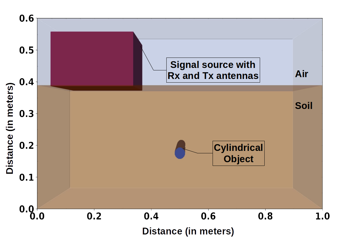
| Sl. No. | Soil Type | (S/m) | permittivity |
| 1 | Dry and sandy | 0.002 | 10 |
| 2 | wooded | 0.0075 | 12 |
| 3 | 0.01 | 15 | |
| 4 | Rocky land, steep hills | 0.002 | 12.5 |
| 5 | (to about 1000 m) | 0.001 | 5 |
| 6 | Pastoral Hills, rich soil | 0.007 | 17 |
| 7 | and forestation | 0.005 | 13 |
| Parameters | Parameter values |
| Source Frequency | 400 MHz |
| Source Waveform | Gaussian |
| Resolution (Spatial) | 2 mm |
| A-Scan intervals | 6 mm |
| No of A-Scans | 108 |
| Time Window | 14 ns |
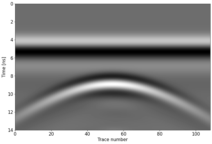
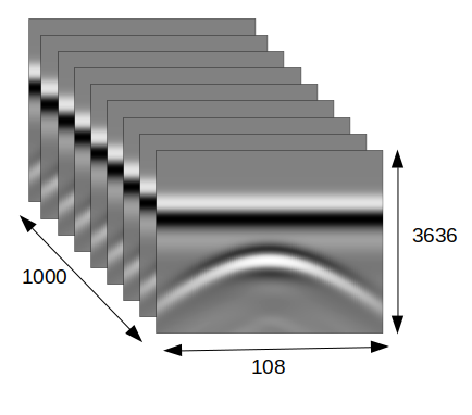
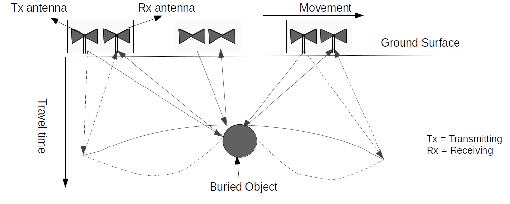
The overall GPR data processing pipeline in this work consists of feature extraction, splitting of dataset into train-test sets, normalising the data, training of CNN model, and validation.
As a means of feature extraction, edge detection is used. There are several operators for edge detection that are used in image processing. In this work, Sobel, Laplacian, Scharr, and Canny operators are used for comparing the performance of the proposed CNN architecture. Hyperbolic curves are one of the distinguishing features in GPR images. The parameters of a hyperbolic signature can be used to estimate the size and location of the related target object in addition to the characteristics of the medium (e.g.: soil). In edge detection we try to find the regions in an image where there is a sharp change in intensity or colour. The higher the value, steeper the change and vice versa.
5.1.1. Sobel OperatorA very common operator for edge detection is a Sobel operator. Sobel is a very popular operator and is widely used by researchers as an edge detection tool ([52]). The Sobel operator is a gradient based method and it calculates the first derivatives of the image separately for the X and Y axes. The derivative in X direction is computed by convolving the image $f(x,y)$ with a kernel $G_x$. For a kernel size of 3, $G_x$ is computed as shown in equation \eqref{eq1}. The derivative in Y direction is computed as shown in equation \eqref{eq2}. \begin{equation} \label{eq1} G_{x} = \begin{bmatrix} -1 & 0 & +1 \\ -2 & 0 & +2 \\ -1 & 0 & +1 \end{bmatrix} * f(x,y) \end{equation} \begin{equation} \label{eq2} G_{y} = \begin{bmatrix} -1 & -2 & -1 \\ 0 & 0 & 0 \\ +1 & +2 & +1 \end{bmatrix} * f(x,y) \end{equation} From equations \eqref{eq1} and \eqref{eq2}, the gradient of an image $f(x,y)$ with respect to x and y directions can be shown as given in equation \eqref{eq1}. The gradient will be in whichever direction the change will be more intense. This gradient direction is calculated as given by equation \eqref{eq2}. Finally, at each pixel of the image, the approximation of the gradient is calculated by equation \eqref{eq3}. \begin{equation} \label{eq3} \nabla f = [G_x, G_y] = \left [ \frac{\partial f}{\partial x},\frac{\partial f}{\partial y} \right ] \end{equation} \begin{equation} \label{eq4} \theta = tan^{-1}\left ( \frac{G_x}{G_y} \right ) = tan^{-1}\left ( \frac{\partial f}{\partial y}/\frac{\partial f}{\partial x} \right ) \end{equation} \begin{equation} \label{eq5} G = \left \| \nabla f \right \| = \sqrt{ G_{x}^{2} + G_{y}^{2} } = \sqrt{\left ( \frac{\partial f}{\partial x} \right )^{2}+\left ( \frac{\partial f}{\partial y} \right )^{2}} \end{equation} In this work, 7$\times$7 Sobel kernels are implemented. By increasing the size of the convolution matrix, the edge detector becomes less sensitive to local noise. This is useful for low contrast images where edges might not be easy to detect. Sobel operator has the advantage of providing edge detection with simultaneous reduction in noise (gaussian smoothing).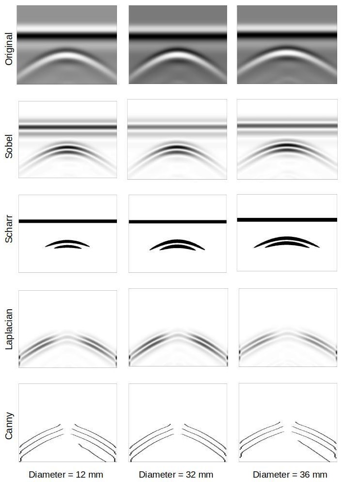
- Noise reduction using a Gaussian filter.
- Calculate intensity gradient using Sobel filter, using equations \eqref{eq4} and \eqref{eq5}.
- Remove unwanted pixels which may not be part of the edges (non-maximum suppression).
- Using high and low threshold intensity values, focus on the edges which are important for the present application and filter out the unwanted pixels which non-maximum suppression could not.
| Sl. No. | Hidden Layers | Validation Loss (MAPE) | ||||
Detector | Sobel | Laplacian | Scharr | Canny | ||
| 1 | 1 Layer | 28.99 | 33.1 | 30.41 | 8.70 | 18.51 |
| 2 | 2 Layers | 29.59 | 30.40 | 31.91 | 9.55 | 19.96 |
| 3 | 3 Layers | 30.84 | 34.46 | 34.27 | 7.72 | 20.16 |
| 4 | 4 Layers | 30.32 | 35.68 | 32.99 | 7.65 | 21.31 |
| 5 | 5 Layers | 16.39 | 31.23 | 29.29 | 6.94 | 23.97 |
| 6 | 6 Layers | 16.34 | 30.56 | 29.25 | 8.71 | 25.58 |
| 7 | 7 Layers | 16.14 | 30.24 | – | 8.35 | – |
| 8 | 8 Layers | 16.55 | – | – | 8.36 | – |
| 9 | 9 Layers | 16.11 | – | – | 8.50 | – |
| 10 | 10 Layers | 20.49 | – | – | 9.87 | – |
NVIDIA RTX3090 GPU was used in CNN training. Using a GPU, the CNN training time reduced from several hours on CPU to less than 1 hour.
The whole GPR data processing pipeline, including the CNN and its optimisation algorithms, is written in Python, along with its image processing extension OpenCV and its deep learning extensions, Keras and TensorFlow.
6. Results and DiscussionIt is observed that the model with Scharr edge detector followed by CNN model with 5 hidden layers performs the best with a validation loss of 6.94 (MAPE). However, Sobel, Laplacian, and Canny edge detectors did not give favourable results with the current dataset. Best MAPE (validation) for the CNN model with Sobel edge detector is 30.24 (7 hidden layers), Laplacian edge detector is 29.25 (6 hidden layers), and Canny edge detector is 18.51 (1 hidden layer).
Since the CNN model with Scharr edge detector shows the best validation loss, its model is saved in HDF5 format to evaluate its performance on other datasets. For a final performance evaluation of the model, another set of 100 B-Scans is created using gprMax. The MAPE of the model for this new and unseen dataset is found to be 7.49. Table 4 shows the performance of the model on the new dataset.
| Sl. No. | value | Prediction | Prediction | Median |
| 1 | 10 | 9.58 | 7.27 | 9.51 |
| 2 | 12 | 13.16 | 17.48 | 14.59 |
| 3 | 14 | 14.18 | 17.18 | 14.18 |
| 4 | 16 | 15.33 | 17.12 | 15.33 |
| 5 | 18 | 19.06 | 21.39 | 20.11 |
| 6 | 20 | 19.53 | 23.45 | 20.95 |
| 7 | 22 | 22.30 | 24.57 | 21.80 |
| 8 | 23 | 24.51 | 24.85 | 24.68 |
| 9 | 24 | 23.93 | 30.25 | 24.51 |
| 10 | 26 | 26.05 | 23.70 | 25.73 |
| 11 | 27 | 32.06 | 32.06 | 32.06 |
| 12 | 28 | 30.59 | 23.46 | 27.32 |
| 13 | 30 | 29.47 | 23.56 | 30.81 |
| 14 | 31 | 32.68 | 35.58 | 34.13 |
| 15 | 32 | 33.33 | 24.89 | 33.73 |
| 16 | 34 | 35.09 | 29.33 | 35.09 |
| 17 | 36 | 36.30 | 39.74 | 36.30 |
| 18 | 38 | 39.70 | 27.72 | 34.86 |
| 19 | 39 | 36.28 | 36.28 | 36.28 |
| 20 | 40 | 40.40 | 37.80 | 39.24 |
A violin plot showing the distribution of predicted values and their probability density is shown in Figure 8. It divides the data points (predicted values) into four equal portions (quartiles). The white dot in the middle denotes the median value and the thick black bar denotes the interquartile range. The thin black line extending on both sides represents the upper and lower adjacent values in the predicted data. The kernel density estimation on both sides of the black line shows the distribution of the data.
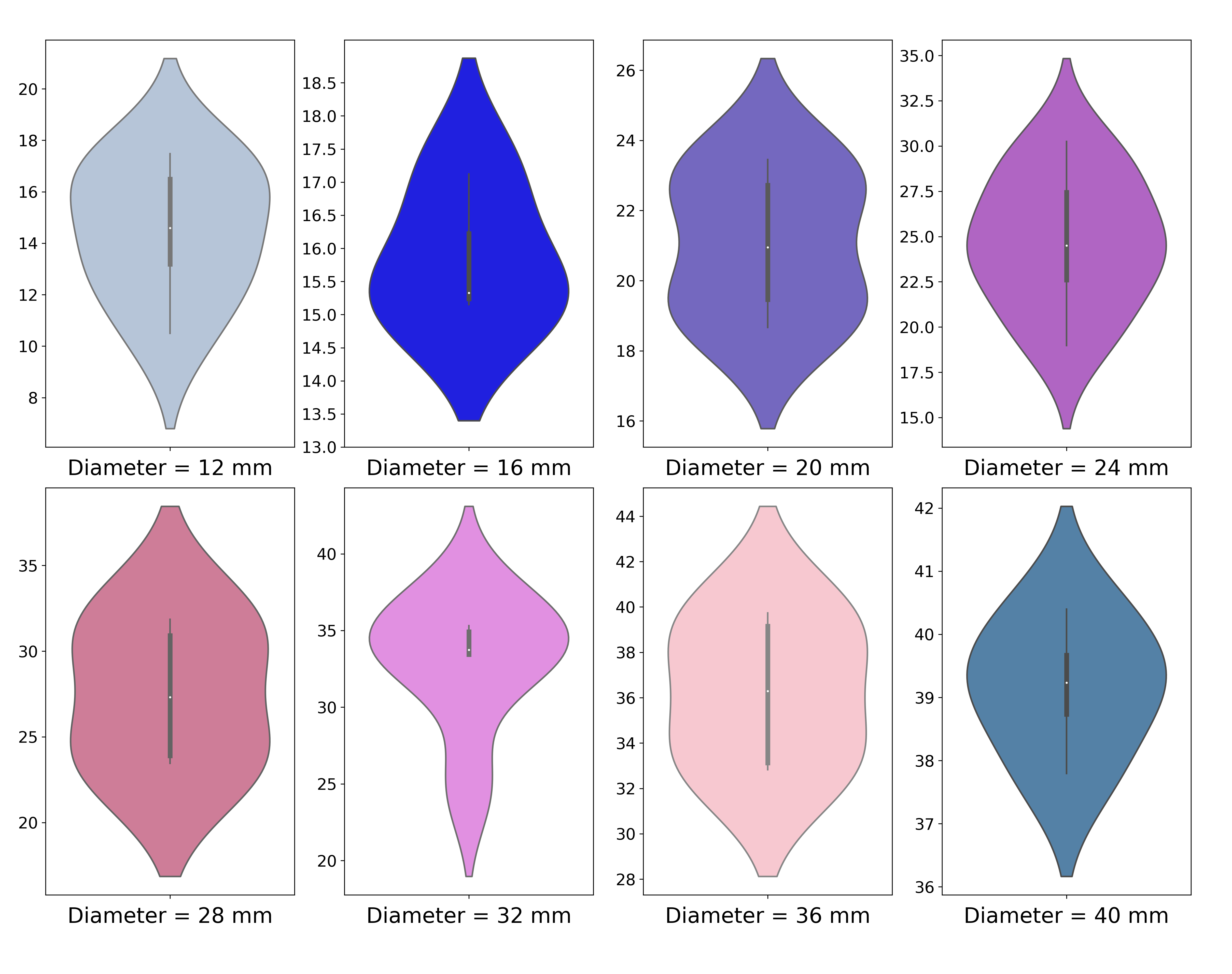
In Figure {8}, the plot for diameter 24 mm shows that the median value of the predicted values is 24.51 mm. For an actual value of 24 mm, the highest predicted value of 30.25 mm and the lowest predicted value of 23.93 mm create the boundaries of the interval space which contains all the data points. The interquartile range (IQR) shows the middle 50% of the four quartiles. In this case, the IQR ranges from 22.5 mm (first quartile) to 27.5 mm (third quartile) which means the middle 50% of the predicted values lie between 22.5 mm to 27.5 mm. The kernel density estimation (KDE) plot shows the probability distribution of the predicted values on both the sides of the vertical black line. The KDE plot goes to a maxima at around 24.51 mm which signifies that the probability of finding a predicted value near to 24.51 mm is maximum. This is in rough agreement with the fact that the actual value is 24 mm.
A comparison of the model’s performance shows that Scharr edge detector (SED) followed by a 6 convolution layer CNN model boosts the overall performance over the other methods used. The SED approach extracts sufficient signature information related to the size of the object to raise the system’s performance and reduce its validation MAPE to 6.74 and a MAPE of 7.49 on new, unseen data.
6.1. Testing on noisy dataGPR images are seldom noise-free and ideal hyperbolic reflections are not obtained in most cases. Hence, it is imperative to test any feature extraction model on noisy data for proper evaluation of its performance in realistic scenarios.
For this, a new dataset is generated by adding noise randomly. Random number of pixels are selected for each GPR B-Scan and replaced with white and black pixels. The total number of pixels in each B-Scan being 3,92,688 (108 $\times$ 3636), the range of the randomly selected pixels is randomly varied from ~0.3% (1400) to ~25% (98000). Before applying the proposed model for diameter prediction, the image is first passed through a median filter which is a widely used non-linear filter to remove noise in GPR images. A Scharr filter is then applied on the image, after which the CNN model is used for diameter prediction. Figure 9 shows a GPR B-Scan with 10% noise added to it. Below it is the noise-free image after a median filter is used.
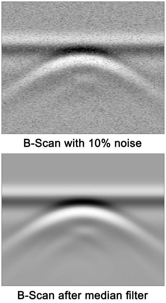
Several images containing various amounts of noise are evaluated using the proposed CNN model. Table 5 shows the performance of the model for different noise levels in the input image. As seen from the table, the model is able to predict the target’s diameter with low error rates at low noise levels. However, as the noise level increases beyond 20%, it is seen that model’s performance degrades with error rates of 22.26% at 20% noise level and upto 26.88% at 25% noise level.
| Sl. No. | Level | Diameter of target object (mm) | (mm) | |
| True values | Predicted values | |||
| 1 | 01% | 36 | 36.92 | 0.92 |
| 2 | 02% | 14 | 14.30 | 0.30 |
| 3 | 03% | 36 | 34.03 | 1.97 |
| 4 | 04% | 18 | 17.75 | 0.25 |
| 5 | 04% | 17 | 17.70 | 0.70 |
| 6 | 04% | 26 | 24.58 | 1.42 |
| 7 | 05% | 22 | 23.58 | 1.58 |
| 8 | 05% | 38 | 34.43 | 3.57 |
| 9 | 05% | 24 | 20.84 | 3.16 |
| 10 | 10% | 18 | 17.35 | 0.65 |
| 11 | 10% | 26 | 24.85 | 1.15 |
| 12 | 10% | 16 | 17.02 | 1.02 |
| 13 | 10% | 28 | 25.47 | 2.53 |
| 14 | 10% | 36 | 32.60 | 3.40 |
| 15 | 15% | 28 | 26.47 | 1.53 |
| 16 | 15% | 30 | 27.66 | 2.34 |
| 17 | 15% | 16 | 14.03 | 1.97 |
| 18 | 15% | 14 | 12.23 | 1.77 |
| 19 | 15% | 26 | 29.80 | 3.80 |
| 20 | 20% | 22 | 20.82 | 1.18 |
| 21 | 20% | 14 | 14.91 | 0.91 |
| 22 | 20% | 36 | 39.37 | 3.37 |
| 23 | 20% | 28 | 21.77 | 6.23 |
| 24 | 20% | 14 | 10.40 | 3.60 |
| 25 | 25% | 20 | 15.58 | 4.42 |
| 26 | 25% | 14 | 10.80 | 3.20 |
| 27 | 25% | 26 | 19.01 | 6.99 |
A CNN model for detecting and predicting the size of buried objects will not be considered for practical application if it can be applied to metallic targets only. Hence, its performance evaluation is needed for non-metallic targets as well. For this purpose, a dataset consisting of PVC ($\sigma$ = 0.001 Siemens/metre, $\epsilon_r$ = 4) and concrete ($\sigma$ = 0.01 Siemens/metre, $\epsilon_r$ = 7.3) is generated. Figure 10 shows a GPR B-Scans after a application of Scharr filter for PVC and concrete targets.
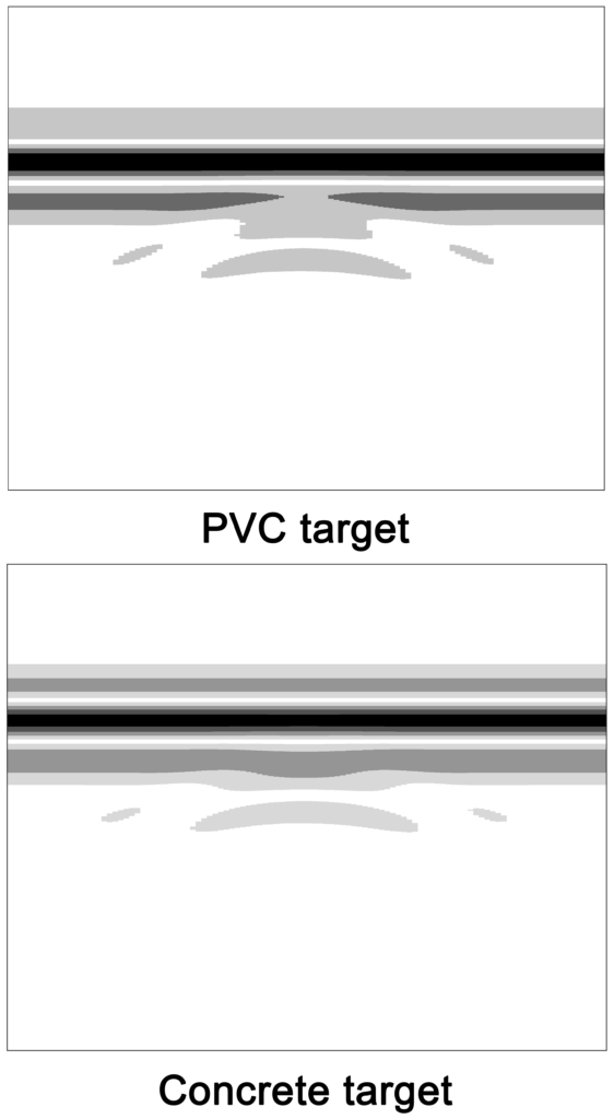
On evaluation of the CNN model of this dataset, it is seen that it can predict the target’s size with very low error rates, irrespective of the target material. The dataset is generated using the methodology as previously described in section Section 2. Table 6 lists the values predicted by the model for different target materials having different sizes.
| Sl. No. | Material | Diameter of target object (mm) | (mm) | |
| True values | Predicted values | |||
| 1 | PVC | 34 | 32.90 | 1.10 |
| 2 | Concrete | 18 | 19.28 | 1.28 |
| 3 | Concrete | 32 | 30.12 | 1.88 |
| 4 | PVC | 16 | 14.91 | 1.09 |
| 5 | Concrete | 26 | 28.39 | 2.39 |
| 6 | PVC | 20 | 21.83 | 1.83 |
| 7 | PVC | 30 | 31.36 | 1.36 |
| 8 | PVC | 10 | 9.79 | 0.21 |
| 9 | Concrete | 18 | 19.38 | 1.38 |
| 10 | PVC | 22 | 20.12 | 1.88 |
| 11 | Concrete | 34 | 32.11 | 1.89 |
| 12 | Concrete | 26 | 23.72 | 2.28 |
| 13 | Concrete | 20 | 18.44 | 1.56 |
| 14 | Concrete | 24 | 24.29 | 0.29 |
| 15 | PVC | 16 | 16.54 | 0.54 |
| 16 | PVC | 16 | 14.76 | 1.24 |
| 17 | Concrete | 38 | 34.59 | 3.41 |
| 18 | Concrete | 28 | 25.87 | 2.13 |
| 19 | Concrete | 28 | 25.41 | 2.59 |
| 20 | Concrete | 30 | 27.29 | 2.71 |
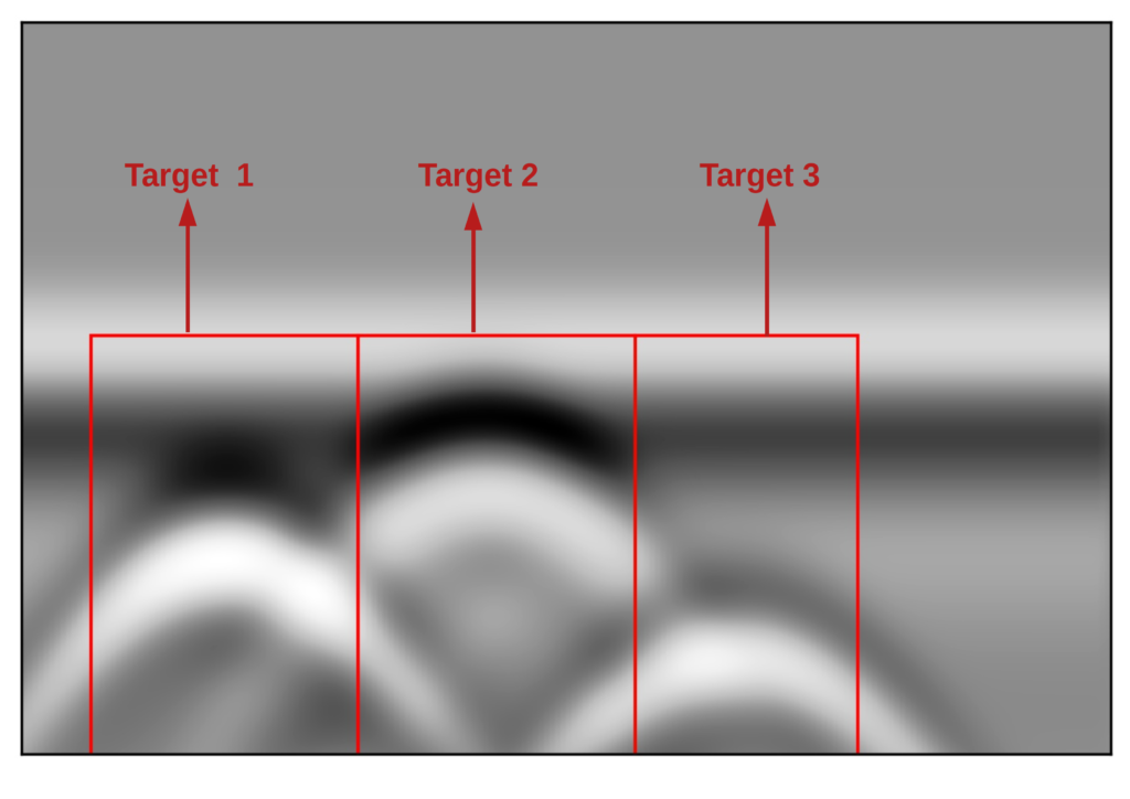
To test the efficacy of the model when multiple buried objects are present, few B-Scans are generated containing upto 3 objects of different sizes and at different depths. All the objects are considered to be cylindrical in shape. One such B-Scan image is shown in Figure 11 where multiple hyperbolas with overlapping edges can be seen. It contains 3 metallic cylinders at depths of diameters 30 mm, 20 mm, and 40 mm from left-to-right.
In the case of multiple target objects, the hyperbolas will have to be isolated from the image before the model can be used for estimation of target size. The hyperbolas can be isolated using template matching, which is a commonly used algorithm in image processing. They can also be extracted manually by cropping the image. Next, each image containing the individual hyperbola is reshaped to have the same size as required by the CNN model, in this case 108 $\times$ 3636. This is done by padding around the edges of each image with linearly varying values from the pixels at the edge of the image to the 3636th / 108th pixel.
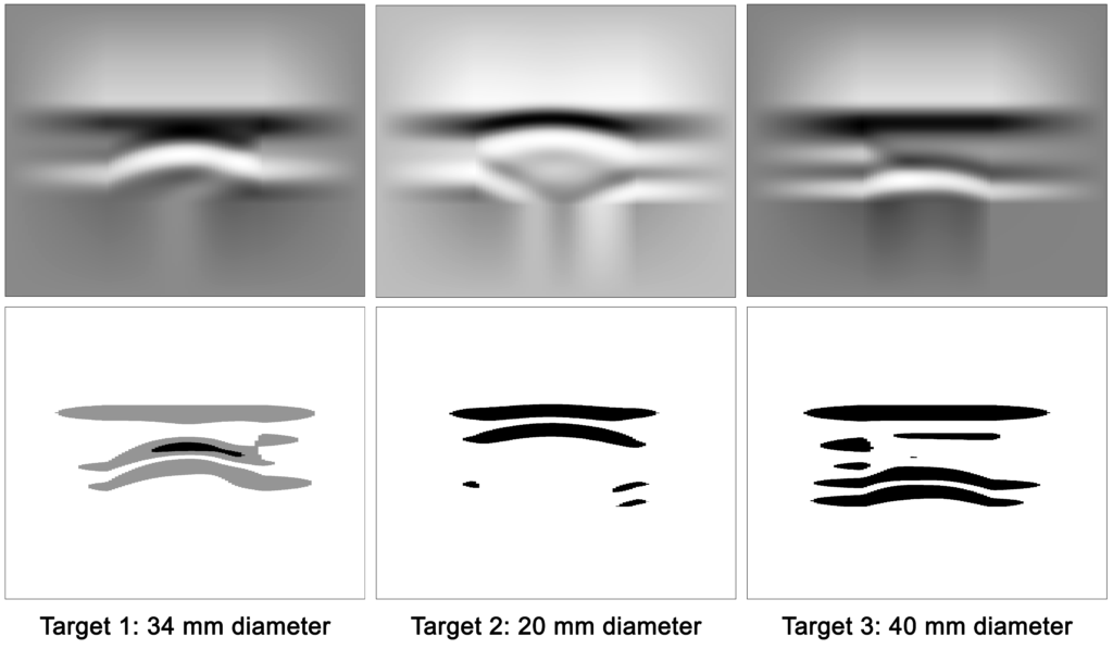
As shown in Figure 12, a Scharr filter is finally applied to each image after which the CNN model is used to estimate the size of the targets. The model shows decent performance in estimating the size of the targets. It predicted a size of 34.46 mm for the object with 34 mm actual diameter, 22.86 mm for 20 mm (actual), and 44.15 mm for an actual diameter of 40 mm. However, those performances in which each image recorded a single hyperbola were better than this result.
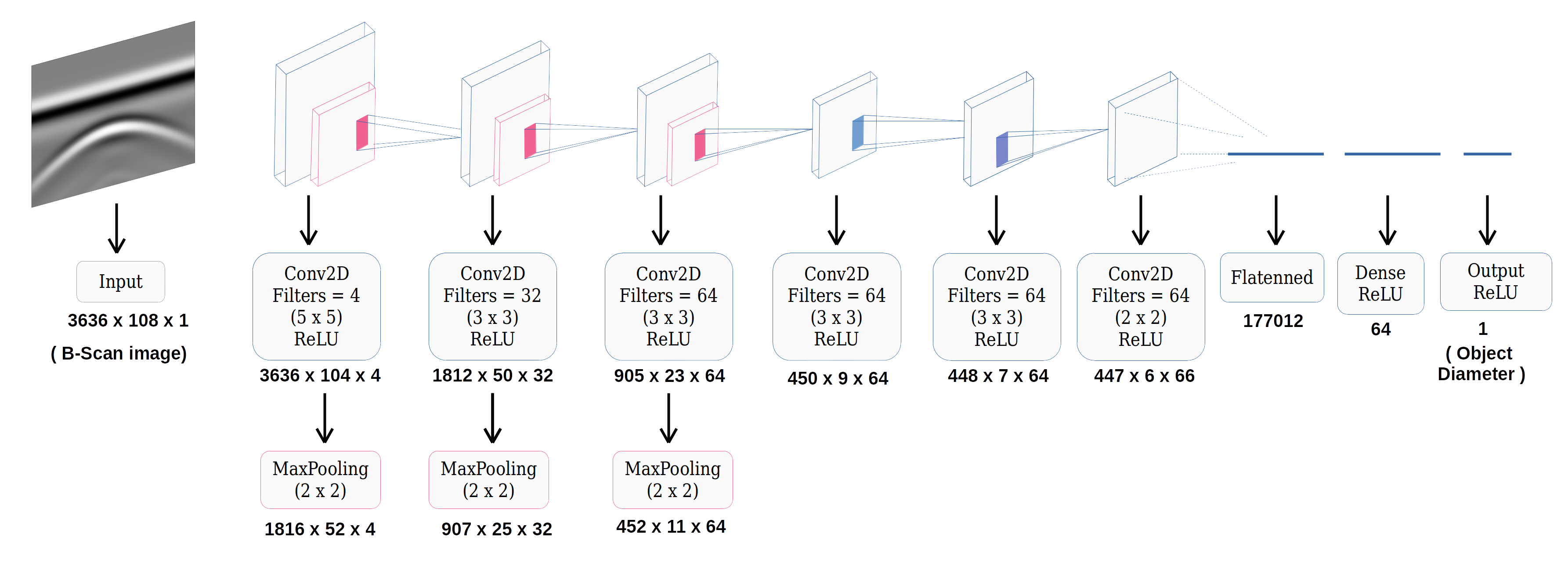
A novel approach of using CNN for predicting size of buried objects from GPR B-Scans was presented. The proposed CNN architecture extracts high level signatures in the first stage of feature extraction and learns additional low level features when the input data passes through the neural network to finally make an estimation of the required parameter. A comparison with other techniques is shown in Table 7 from which it can be concluded that the application of CNN in this problem has demonstrated a good performance in predicting size of buried objects. Moreover, it can be used in real time applications in GPR data interpretation since such a model can be implemented on embedded devices like ARM, FPGA, etc.
No. | Author | Technique used | Application | Offline |
| 1 | Chaudhuri and Samanta (1991) ([12]) | Hyperbolic feature extraction using Moment of inertia optimisation | Extraction of hyperbolic features | Offline |
| 2 | Delbo et al. (2000) [11] | Hyperbolic feature extraction using Fuzzy shell clustering | Extraction of hyperbolic features | Offline |
| 3 | Ko et al. (2012) [3] | PCA and Fourier Transform | Detection of landmines | Offline |
| 4 | Wahab et al. (2013) [2] | Hyperbola fitting technique | Estimation of radius of pipes and cables | Offline |
| 5 | Maas and Schmalzl (2013) [13] | Canny operator for edge detection and Hough transform for hyperbola fitting | Automatically localize reflection hyperbola | Real time |
| 6 | Besaw and Stimac (2015) [28] | ANN based Deep Belief Network (DBN) | Detection of explosive hazards | Offline (in situ) |
| 7 | Mertens et al. (2015) [9] | Hyperbolic feature extraction using Canny operator | Automated detection of reflection hyperbola | Offline |
| 8 | Dou et al. (2016) [14] | Canny operator for edge detection and Hough transform for hyperbola fitting | Automatically localize reflection hyperbola | Real time |
| 9 | Li et al. (2016) [8] | Hyperbolic feature extraction using Sobel operator followed by Hough Transform | Automatic recognition of tree roots | Offline |
| 10 | Lameri et al. (2017) [29] | Deep Convolutional Neural Network | Detection of landmines | Real Time |
| 11 | Todkar et al. (2017) [56] | Machine learning using Support Vector Machines (SVM) | Detection of debondings | Offline (in situ) |
| 12 | Kafedziski et al. (2018) [32] | Faster Region Convolutional Neural Network (Faster R-CNN) | Detection and classification of landmines | Real Time |
| 13 | Sonoda and Kimoto (2018) [57] | Deep CNN | Object identification | Real Time |
| 14 | Kang et al. (2020) [58] | Basis pursuit-based background filtering algorithm followed by deep CNN | Underground cavity detection | Real Time |
| 15 | Bugarinović et al. (2020) [10] | Hyperbolic feature extraction using Canny operator | Automated detection of hyperbolic features | Offline |
| 16 | Giannakis et al. (2021) [33] | Autoencoder as a pre processing step followed by ANN based regressor | Estimate the diameter of reinforcement bars in concrete | Real Time |
| 17 | Present work | Hyperbolic feature detection followed by deep CNN | Estimation of radius/ diameter of buried objects | Real time |
Future work of this approach will concentrate on experimentally verifying the model with actual data taken from an FPGA-based GPR system being developed in-house as well as from commercial GPR systems. The present model was trained with an object which is a metallic cylinder made of aluminium. Even though the model was tested on PVC and concrete objects with good results, its performance can still be improved by training it using greater number of datasets containing objects of a variety of materials. Different types of materials will have different dielectric properties and hence will generate different scattering and dispersion characteristics. Similarly, training the model for different shapes such as rectangular and triangular forms give make it more robust. It remains to be seen how these will affect the robustness of the proposed approach.
8. Acknowledgements The authors would also like to thank Dr. Manoj Kumar Phukan (Sr. Scientist, Geo Sciences and Technology Division, CSIR-NEIST, Jorhat) who gave detailed insights on interpretation of GPR data and Ms. Sharmistha Mazumdar for her help in visualising the results. Finally, the authors appreciate the help of Mr. Arnob Doloi for his inputs during database creation from time to time. The authors would also like to thank Ms. Sweta Kumar Gaur for her insightful suggestions in linguistic polish of the manuscript. 9. Data Availability All the data, models, or codes generated during this study are available from the corresponding author upon request.References
- (2013): Histograms of oriented gradients for landmine detection in ground-penetrating radar data. In: IEEE transactions on geoscience and remote sensing, vol. 52, no. 3, pp. 1539–1550, 2013.
- (2013): Interpretation of Ground Penetrating Radar (GPR) image for detecting and estimating buried pipes and cables. In: 2013 IEEE International Conference on Control System, Computing and Engineering, pp. 361–364, IEEE, 2013.
- (2012): GPR-based landmine detection and identification using multiple features. In: International journal of antennas and propagation, vol. 2012, 2012.
- (2004): Detection of linear objects in GPR data. In: Signal Processing, vol. 84, no. 4, pp. 785–799, 2004.
- (2005): The estimation of buried pipe diameters using ground penetrating radar. In: Insight-Non-Destructive Testing and Condition Monitoring, vol. 47, no. 7, pp. 394–399, 2005.
- (2010): Probabilistic robust hyperbola mixture model for interpreting ground penetrating radar data. In: pp. 1–8, 2010.
- (2019): Non-invasive estimation of root zone soil moisture from coarse root reflections in ground-penetrating radar images. In: Plant and Soil, vol. 436, no. 1-2, pp. 623–639, 2019.
- (2016): Tree root automatic recognition in ground penetrating radar profiles based on randomized Hough transform. In: Remote Sensing, vol. 8, no. 5, pp. 430, 2016.
- (2015): Automated detection of reflection hyperbolas in complex GPR images with no a priori knowledge on the medium. In: IEEE Transactions on Geoscience and Remote Sensing, vol. 54, no. 1, pp. 580–596, 2015.
- (2020): On the Introduction of Canny Operator in an Advanced Imaging Algorithm for Real-Time Detection of Hyperbolas in Ground-Penetrating Radar Data. In: Electronics, vol. 9, no. 3, pp. 541, 2020.
- (2000): A fuzzy shell clustering approach to recognize hyperbolic signatures in subsurface radar images. In: IEEE Transactions on Geoscience and Remote Sensing, vol. 38, no. 3, pp. 1447–1451, 2000.
- (1991): Elliptic fit of objects in two and three dimensions by moment of inertia optimization. In: Pattern Recognition Letters, vol. 12, no. 1, pp. 1–7, 1991.
- (2013): Using pattern recognition to automatically localize reflection hyperbolas in data from ground penetrating radar. In: Computers & geosciences, vol. 58, pp. 116–125, 2013.
- (2016): Real-time hyperbola recognition and fitting in GPR data. In: IEEE Transactions on Geoscience and Remote Sensing, vol. 55, no. 1, pp. 51–62, 2016.
- (2016): Ground-penetrating radar velocity determination and precision estimates using common-midpoint (CMP) collection with hand-picking, semblance analysis and cross-correlation analysis: a case study and tutorial for archaeologists. In: Archaeometry, vol. 58, no. 6, pp. 987–1002, 2016.
- (2016): Development of an analytic approach utilizing the extended common midpoint method to estimate asphalt pavement thickness with 3-D ground-penetrating radar. In: NDT & E International, vol. 78, pp. 29–36, 2016.
- (2020): Target detection using supervised machine learning algorithms for GPR data. In: Sensing and Imaging, vol. 21, no. 1, pp. 1–15, 2020.
- (2008): Detection and discrimination of land mines in ground-penetrating radar based on edge histogram descriptors and a possibilistic $ k $-nearest neighbor classifier. In: IEEE Transactions on Fuzzy Systems, vol. 17, no. 1, pp. 185–199, 2008.
- (2012): An approach for predicting the shape and size of a buried basic object on surface ground penetrating radar system. In: International Journal of Antennas and Propagation, vol. 2012, pp. 1–13, 2012.
- (2014): Feature extraction and automatic material classification of underground objects from ground penetrating radar data. In: Journal of Electrical and Computer Engineering, vol. 2014, 2014.
- (2002): Image processing and neural network techniques for automatic detection and interpretation of ground penetrating radar data. In: Proceedings of the 6th International Multi-Conference on Circuits, Systems, Communications and Computers, Cancun, Mexico, pp. 12–16, 2002.
- (2017): Point coordinates extraction from localized hyperbolic reflections in GPR data. In: Journal of Applied Geophysics, vol. 144, pp. 1–17, 2017.
- (2000): Automatic detection of buried utilities and solid objects with GPR using neural networks and pattern recognition. In: Journal of applied Geophysics, vol. 43, no. 2-4, pp. 157–165, 2000.
- (2000): Neural detection of pipe signatures in ground penetrating radar images. In: IEEE Transactions on Geoscience and Remote Sensing, vol. 38, no. 2, pp. 790–797, 2000.
- (2005): Location of steel reinforcement in concrete using ground penetrating radar and neural networks. In: Ndt & E International, vol. 38, no. 3, pp. 203–212, 2005.
- (2015): Deep learning applications and challenges in big data analytics. In: Journal of Big Data, vol. 2, no. 1, pp. 1, 2015.
- (2012): Imagenet classification with deep convolutional neural networks. In: Advances in neural information processing systems, pp. 1097–1105, Neural Information Processing Systems Foundation, 2012.
- (2015): Deep convolutional neural networks for classifying GPR B-scans. In: Detection and Sensing of Mines, Explosive Objects, and Obscured Targets XX, pp. 945413, International Society for Optics and Photonics, 2015.
- (2017): Landmine detection from GPR data using convolutional neural networks. In: 2017 25th European Signal Processing Conference (EUSIPCO), pp. 508–512, IEEE, 2017.
- (2016): gprMax: Open source software to simulate electromagnetic wave propagation for Ground Penetrating Radar. In: Computer Physics Communications, vol. 209, pp. 163–170, 2016.
- (2016): Underground object characterization based on neural networks for ground penetrating radar data. In: Yu, Tzuyang; Gyekenyesi, Andrew L.; Shull, Peter J.; Wu, H. Felix (Ed.): Nondestructive Characterization and Monitoring of Advanced Materials, Aerospace, and Civil Infrastructure 2016, pp. 10 – 18, International Society for Optics and Photonics SPIE, 2016.
- (2018): Detection and classification of land mines from ground penetrating radar data using faster R-CNN. In: 2018 26th Telecommunications Forum (TELFOR), pp. 1–4, IEEE, 2018.
- (2020): A machine learning scheme for estimating the diameter of reinforcing bars using ground penetrating radar. In: IEEE Geoscience and Remote Sensing Letters, 2020.
- (2016): Convolutional neural network with data augmentation for SAR target recognition. In: IEEE Geoscience and remote sensing letters, vol. 13, no. 3, pp. 364–368, 2016.
- (2016): Target classification using the deep convolutional networks for SAR images. In: IEEE Transactions on Geoscience and Remote Sensing, vol. 54, no. 8, pp. 4806–4817, 2016.
- (2018): Innovative method for recognizing subgrade defects based on a convolutional neural network. In: Construction and Building Materials, vol. 169, pp. 69–82, 2018.
- (2018): Characterization and identification of asphalt mixtures based on Convolutional Neural Network methods using X-ray scanning images. In: Construction and Building Materials, vol. 174, pp. 72–80, 2018.
- (2017): A new method to determine locations of rebars and estimate cover thickness of RC structures using GPR data. In: Construction and Building Materials, vol. 140, pp. 257–273, 2017.
- (2020): Detection and localization of rebar in concrete by deep learning using ground penetrating radar. In: Automation in Construction, vol. 118, pp. 103279, 2020.
- (2009): Gaussian process approach to buried object size estimation in GPR images. In: IEEE Geoscience and Remote Sensing Letters, vol. 7, no. 1, pp. 141–145, 2009.
- (2019): A CUDA-based GPU engine for gprMax: Open source FDTD electromagnetic simulation software. In: Computer Physics Communications, vol. 237, pp. 208–218, 2019.
- (1954): Dielectric Materials and Applications; papers by twenty-two contributors. published jointly by the Technology Press of M.I.T. and Wiley, 1954.
- (2015): A review on computer vision based defect detection and condition assessment of concrete and asphalt civil infrastructure. In: Advanced Engineering Informatics, vol. 29, no. 2, pp. 196–210, 2015.
- (2017): Image based techniques for crack detection, classification and quantification in asphalt pavement: a review. In: Archives of Computational Methods in Engineering, vol. 24, no. 4, pp. 935–977, 2017.
- (2013): Automatic quantification of crack patterns by image processing. In: Computers & Geosciences, vol. 57, pp. 77–80, 2013.
- (2014): Image-based retrieval of concrete crack properties for bridge inspection. In: Automation in construction, vol. 39, pp. 180–194, 2014.
- (2012): An Unmanned Aerial Vehicle-Based Imaging System for 3D Measurement of Unpaved Road Surface Distresses 1. In: Computer-Aided Civil and Infrastructure Engineering, vol. 27, no. 2, pp. 118–129, 2012.
- (2020): 3D CNN-PCA: A deep-learning-based parameterization for complex geomodels. In: Computers & Geosciences, pp. 104676, 2020.
- (2017): Angel-Eye: A complete design flow for mapping CNN onto embedded FPGA. In: IEEE Transactions on Computer-Aided Design of Integrated Circuits and Systems, vol. 37, no. 1, pp. 35–47, 2017.
- (2019): A high-throughput and power-efficient FPGA implementation of YOLO CNN for object detection. In: IEEE Transactions on Very Large Scale Integration (VLSI) Systems, vol. 27, no. 8, pp. 1861–1873, 2019.
- (2018): Automated detection of sewer pipe defects in closed-circuit television images using deep learning techniques. In: Automation in Construction, vol. 95, pp. 155–171, 2018.
- (2020): Radar remote sensing image retrieval algorithm based on improved Sobel operator. In: Journal of Visual Communication and Image Representation, vol. 71, pp. 102720, 2020.
- (1987): Edge Focusing. In: IEEE Transactions on Pattern Analysis and Machine Intelligence, vol. PAMI-9, no. 6, pp. 726–741, 1987.
- (2014): Gray-level transformation and Canny edge detection for 3D seismic discontinuity enhancement. In: Computers & Geosciences, vol. 72, pp. 192–200, 2014.
- (2017): Nesterov's accelerated gradient and momentum as approximations to regularised update descent. In: 2017 International Joint Conference on Neural Networks (IJCNN), pp. 1899–1903, IEEE 2017.
- (2017): Detection of debondings with ground penetrating radar using a machine learning method. In: 2017 9th International Workshop on Advanced Ground Penetrating Radar (IWAGPR), pp. 1–6, IEEE 2017.
- (2018): Object identification form GPR images by deep learning. In: 2018 Asia-Pacific Microwave Conference (APMC), pp. 1298–1300, IEEE 2018.
- (2020): Deep learning-based automated underground cavity detection using three-dimensional ground penetrating radar. In: Structural Health Monitoring, vol. 19, no. 1, pp. 173–185, 2020.
