Classification of Soil Types from GPR B-Scans using Deep Learning Techniques

Authors

Nairit Barkataki^*, Sharmistha Mazumdar^*, P Bipasha Devi Singha⁺, Jyoti Kumari⁺, Banty Tiru^# and Utpal Sarma^*

* Dept of Instrumentation & USIC, Gauhati University, Guwahati, India
+ Department of Computer Science, Handique Girls’ College, Guwahati, India
# Dept of Physics, Gauhati University, Guwahati, India

Keywords. deep learning, classification, soil type, ground penetrating radar

---

Note:

This article was published in RTEICT 2021. You may cite the article using the following bibliographic data:

© 2021 IEEE. Personal use of this material is permitted. Permission from IEEE must be obtained for all other uses, in any current or future media, including reprinting/republishing this material for advertising or promotional purposes, creating new collective works, for resale or redistribution to servers or lists, or reuse of any copyrighted component of this work in other works.

---

Contents
Contents
 1.  Introduction
 2.  GPR Data
   2.1.  Database Creation
   2.2.  Data preprocessing
 3.  Methodology
   3.1.  Hyper-parameters
   3.2.  Cross Validation
   3.3.  The proposed model
 4.  Results
 5.  Conclusion
   5.1.  Limitations
   5.2.  Future Work
 6.  Acknowledgement
1. Introduction

Soil consists of different materials and change in the composition and proportion of these materials leads to variation in soil properties. Identification of soil types helps in making conscious decisions regarding farming practices. Knowledge about soil is crucial in agro-electronics for development of various instruments.

Traditionally, soil investigations were done by pedologists observing morphological characteristics combined with laboratory measurements. Before any construction work, it is imperative to identify the soil classes upto a certain depth. It gives an estimation of the bearing capacity of the soil. The most basic method to identify soil types is to drill boreholes and test soil samples. However, this is time consuming and expensive.

Therefore, development of simple techniques to measure the properties of soil is of vital importance. Moreover, determination of soil type has applications in electromagnetic (EM) wave propagation analysis, subsurface imaging etc. Classification of soil type is sometimes done on the basis of soil permittivity and moisture estimation. There are different methods for this which include time-domain reflectometry (TDR) ^[1], ground-penetrating radar (GPR) measurements ^[2], and remote sensing ^[3].

Non-invasive methods for soil classification and analysis are essential for quick and reliable results. Salam et al. developed a method for real-time in-situ estimation of soil properties (relative permittivity and moisture) using underground transmitter and receiver link in wireless underground communications (WUC) ^[4]. Teng et al. proposed a method for soil classification of using visible–near infrared (vis–NIR) spectroscopy, and digital soil class mapping (DSM) ^[5].

Karim et al. studied on the soil profiles in Moramo River Basin using images from ALOS AVNIR-2 (satellite images) and identification of 11 soil subgroups were done ^[6]. However, remote sensing methods are limited to depths of 20-30 cms.

However, the classification procedure is manual in most cases and requires expertise. It is also time consuming and sometimes subjective. Hence, there is a need to automate this procedure. This is where machine learning comes into the picture ^[7]. Rahman et al. used soil samples collected from Khulna district, Bangladesh and proposed a machine learning model to predict 11 soil series along with land type (class) to identify suitable crop for cultivation ^[8].

Post processing of GPR data is dependant on the soil type of the survey area. In addition to the operating frequency of the system ^[9], soil with high conductivity limits the depth of investigation and diminishes the subsurface features ^[10].

Relative permittivity and conductivity of soil changes with soil types and specific terrain conditions i.e. moisture, vegetation and compactness ^[11]. As a non-destructive method, GPR can be used to determine soil types based on their properties like permittivity, conductivity, soil water content, texture etc. GPR uses electromagnetic waves and measures the reflections caused due to changes in electromagnetic properties of the subsurface environment ^[12]. Liu et al. used GPR to determine soil characteristics and crop root measurements ^[13].

The reflections measured by a GPR, also known as radargrams, are hyperbolic patterns which depend on the electromagnetic properties of the subsurface. Hyperbolic signatures are used in object detection. Lei et al. proposed a deep learning framework to detect hyperbolic signatures from B-Scan images identify buried object by localising hyperbolic regions ^[14].

Takahashi et al. characterised the electromagnetic properties of four soil types using laboratory based methods. Test beds were prepared using the 4 soil types where metal pieces along with bullets, cartridges and landmines were buried and GPR data was collected. Their study concluded that soil properties clearly affected the detection rates of buried objects ^[15].

Shihab et al. applied curve fitting procedures to estimate the radius of subsurface cylindrical objects. They also concluded that accurate estimation of relative permittivity was possible by analysing the radargrams from cylinders of varying radii ^[16]. Mechbal et al. applied post processing on raw GPR data to determine the size of concrete rebars ^[17] while others used machine learning techniques for detecting landmines ^[18] and estimating the size of buried objects ^[19].

Aim of Present Work

Although many remote sensing techniques are used for soil classification and identification of soil properties, more work needs to be done to explore the possibility of classifying soil types based on GPR data. This paper mainly focuses on

1. Creation of a synthetic GPR database for use in classification of 7 different soil types.
2. Development of a deep learning model to classify the above 7 different soil types with a high degree of accuracy.

2. GPR Data 2.1. Database Creation The database is created using an open source electromagnetic simulator, gprMax, developed by the researchers of The University of Edinburgh, United Kingdom. For numerical modelling of GPR, it simulates electromagnetic wave propagation using Finite-Difference Time-Domain (FDTD) method ^[20]. For simulating the models, the model size is considered to be $1000mm\times148mm\times400mm$ ($X\times Y\times Z$). The total height of the model is 400mm, of which the top 50 mm is a layer of air and below it is a 350mm layer of soil. A cylindrical object made of aluminium ($\varepsilon_r$ = 10.8 and $\sigma$ = $3.5\times10^7$ S/m) is buried underneath the soil surface. The radius of the cylinder is changed from 10 mm to 55 mm with increment of 5 mm (10 mm, 15 mm, 20 mm etc.) and values for object depth are 104 mm, 134 mm, 164 mm, 194 mm, 224 mm, 284 mm, 314 mm, 344 mm. A total of 700 different scenarios are created for 7 different soil types using the parameters in Table I.

Sl. No.	Soil Type	Class	Relative permitivity ${\epsilon }_r$	Conductivity $\sigma$ (S/m)
1	Dry, sandy, flat (coastal)	Soil Type 1	10	0.002
2	Marshy, forested, flat	Soil Type 2	12	0.008
3	Mountainous/hilly (to about 1000 m)	Soil Type 3	5	0.001
4	Pastoral Hills, rich soil	Soil Type 4	17	0.007
5	Pastoral medium hills and forestation	Soil Type 5	13	0.005
6	Rich agricultural land (low hills)	Soil Type 6	15	0.01
7	Rocky land, steep hills	Soil Type 7	12.5	0.002

The parameters used for the FDTD simulation are given in Table II. .

Sl. No.	Simulation Parameters	Values
1	Excitation Waveform type	Gaussian
2	Frequency	1500 MHz
3	Spatial Resolution	2mm
4	A-Scans interval	5mm
5	Number of A-Scans	100

The time window should be large enough for the EM waves to travel from the transmitting antenna through the soil and reflected to the receiver. The time window required by the EM waves also depends upon the relative permittivity of the media. The different values of time window required corresponding to different soil properties ($\varepsilon_r$) are given in Table III.

Sl. no.	Relative Permittivity ${\epsilon }_r$	Time window (ns)
1	5	7
2	10	9
3	12, 12.5, 13	10
4	15, 17	11

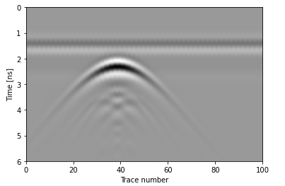
NVIDIA GPUs- P100, Tesla T4, K80 & P4 are used for accelerating all the simulations using the NVIDIA CUDA programming environment. Depending upon the GPU allotted, time taken for each simulation ranges from 30 to 58 minutes. Each B-Scan consists of 100 A-Scans so that the reflections from the buried object are completely visible. Figure 1 shows a B-Scan of an object (cylinder) of radius = 20mm buried at a depth of 194mm from the soil surface having soil type Marshy, forested, flat ($\varepsilon_r$ = 12, $\sigma$ = 0.008 S/m)

2.2. Data preprocessing A total of 700 B-Scans are generated using gprMax. The B-Scan output files are in HDF5 format. Since the B-Scans were generated using different time window values, they have different row numbers varying from 1300 to 3377. To enable easier feeding to the neural network, all B-Scans are made to have equal sizes by adding padding to the smaller images. All 700 B-Scans are then are concatenated along a third dimension to form a 3D numpy having dimensions $700\times3377\times100$. The dataset has a total of $\sim$236 million data points. The array is finally saved to a npz file along with their corresponding labels i.e the soil types. NPZ is a compressed version of the popular npy file format. This helps reduce the size of the synthetic GPR dataset from 4.2 GB to 394 MB. 85% of the dataset is kept for training and validation of the CNN model while 15% is kept for final testing. Since the B-Scans has large feature variations, the data is normalised before using it for any further processing. 3. Methodology In this work, a deep convolutional neural network (CNN) is used for classification of soil types. A 5-fold cross validation is used to train and validate the model. The model’s performance is finally tested on the test set which is totally isolated during the training process. In convolutional neural network (CNN), multiple filters are used by a single convolutional layer to perform convolution of an array over the given image. These filters can identify different features from an image. Adding more such layers increases the capability of the network to extract more complex features ^[21]. The convolved feature size are further reduced using pooling layers. 3.1. Hyper-parameters An optimal combination of hyper-parameters such as number of filters, activation function, learning rate etc. gives the best performing CNN model. But learning the features from data and validating it on the same data (train set) can lead to overfitting of the model. An overfitted model will have poor performance when tested on an unseen dataset. Cross validation is a technique used to prevent overfitting of the model, get the optimal combination of the hyper-parameters and improve its performance.

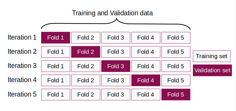
3.2. Cross Validation K-fold is the most commonly used cross validation technique. Here, a test set is kept aside for the final evaluation of the model and the training set is randomly split into k smaller sets of equal size. For each of the k-folds, k-1sets are used to train the model and the resulting model is validated using the one set that is left. The performance of the model is evaluated by the average of all the k accuracies resulting from k-fold cross validation. The visualisation of 5-fold cross validation is shown in Figure 2. Initially, the model is trained for different number of hidden layers. The cross validation score of each model is given in Table IV.

Sl. No.	Number of Hidden Layers	Cross Validation Score
1	3 Layers	74.82%
2	4 Layers	93.90%
3	5 Layers	96.97%

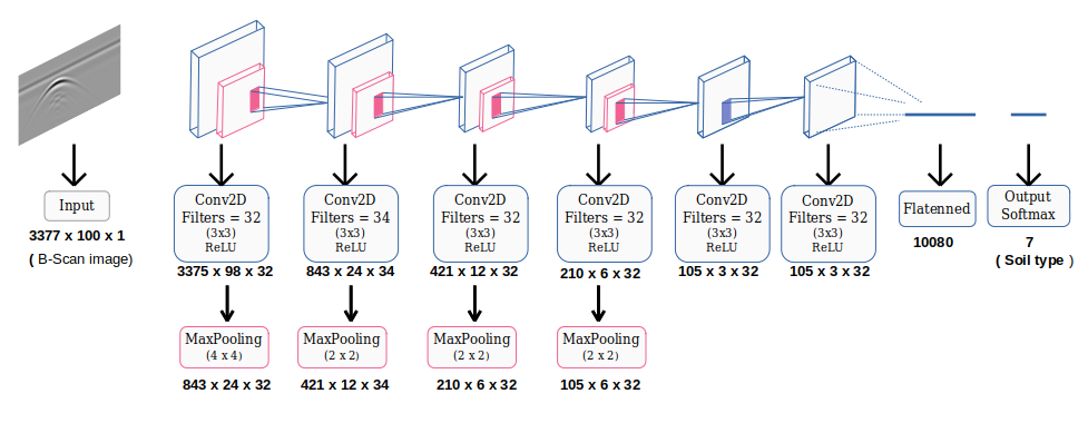
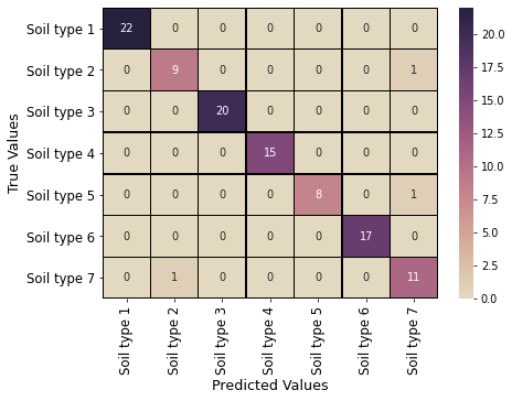
3.3. The proposed model Through multiple training runs, it is seen that the best cross validation accuracy is obtained for the CNN model having 5 hidden layers and the sequence of the layers are shown in Figure 3. There are a total of 6 convolutional layers in the proposed CNN model of which one is the input layer. The activation function used in all the convolutional layers is Rectified Linear Unit (ReLU) which can be defined as ^[21], \begin{equation} \label{eq1} f(x) = max(0,x) \end{equation} ,where x is an input to a neuron. The activation function f(x) gives an output as 0, if x is less than 0 and the output is x (input) otherwise. 32 filters of kernel size $3\times3$ is used in the input layer followed by a MaxPool layer of pool size $4\times4$. Three pairs of convolutional-pooling layer are used after the input layer with filter numbers 34, 32 and 32 respectively. The kernel size of the convolutional layers is $2\times2$ and pool size is $2\times2$ for all pooling layers. Two more convolutional layers are used having the same number of filters and kernel size as the previous layers. After the output from the layer is transformed into a 1D matrix using a flattened layer, 7 neurons are employed in the output layer, to classify the 7 different soil types in the Table I using softmax activation function, mainly used for multi-class classification problems. Adaptive Moment Estimation (Adam) optimisation algorithm is employed in the proposed CNN model with categorical cross-entropy loss function, to reduce the loss function by adjusting the parameters of the model. The whole GPR data processing pipeline are written in Python and its deep learning extensions Keras and TensorFlow. NVIDIA GPU RTX3090 is used for training the CNN model. 4. Results Upon training and validation of the CNN model and then evaluating its performance on unseen data, Table V shows the performance of the model based on the 7 different soil classes. The overall accuracy is 97%. The confusion matrix of the model is shown in Figure 4 in which the y-axis corresponds to the true class labels and the x-axis corresponds to the predicted class labels.

Soil Type	precision	f1-score	recall	accuracy
Soil type 1	1.00	1.00	1.00
Soil type 2	0.90	0.90	0.90
Soil type 3	1.00	1.00	1.00
Soil type 4	1.00	1.00	1.00	0.97
Soil type 5	1.00	0.94	0.89
Soil type 6	1.00	1.00	1.00
Soil type 7	0.85	0.88	0.92

From Figure 4, out 13 images it is seen that, 11 are correctly predicted as having Soil type 7 and remaining 2 incorrectly assigned to other classes. So the precision of Soil type 7 class shown in Table V, can be calculated as \eqref{eq2}, \begin{equation}\label{eq2} Precision = \frac{TP}{TP+FP} = \frac{11}{13} = 0.85 \end{equation} Recall is a statistical metric which tells us how many of the positive instances actually belong to the predicted class. For Soil type 7 in Figure 4, out of the total 12 images actually labelled as Soil type 7, 11 images are correctly predicted and 1 of them is wrongly predicted. So, recall for Soil type 7 can be calculated as \eqref{eq3}, \begin{equation}\label{eq3} Recall = \frac{TP}{TP+FN} = \frac{11}{12} = 0.92 \end{equation} F1 score gives the information of the false predictions of the model, where 1 indicates the best score and 0 indicates the worst score. It is measured using precision and recall. For Soil type 7, f1 score can be calculated as \eqref{eq4}, \begin{equation}\label{eq4} F1~score=2\times\frac{precision\times recall}{precision+recall} = 0.88 \end{equation} 5. Conclusion A novel approach for classifying soil types based on their electromagnetic properties was presented in this paper. A deep CNN model is proposed which is used to classify soil types from GPR B-Scan data. The overall performance of the model can be analysed from confusion matrix in Figure 4 and the classification report in Table V. It is seen that, the classifier is able to correctly classify all images related to soil types 1, 3, 4, 5 and 6 (precision = 1.0) while there are no wrong classifications for soil types 1, 3, 4 and 6 (recall = 1.0). A comparison with other techniques is shown in Table VI. It can be concluded that the proposed CNN model has demonstrated its ability to correctly classify soil types from GPR B-Scans with a high degree of accuracy. The proposed model can be used for automatic classification of soil types and the GPR systems can be calibrated accordingly best penetrate depth and minimum noise.

Sl. No.	Authors	Technique used	Invasive / Non Invasive	Classification Accuracy
1	Harlianto et al. (2017) [22]	SVM based model used to classify soil types. Soil samples collected using hand boring and tested in laboratory	Invasive	82%
2	Rahman et al. (2018) [8]	SVM based model used to classify soil types from soil series data obtained from laboratory measurements	Invasive	94%
3	Inazumi et al. (2020) [23]	CNN based model used to classify pictures of soil samples	Non Invasive	77%
4	Present work	CNN based model used to classify soil types from GPR data	Non Invasive	97%

5.1. Limitations The proposed CNN architecture is trained and tested on a comparatively small dataset. Only 7 different types of soil is considered for this work and real life scenarios might have different combinations of soil. Moreover, the model is yet to be tested on real data. 5.2. Future Work The authors plan to improve the proposed model by:

• Generating more data using different soil properties and for different target materials.
• Implementing the proposed model on real data.

6. Acknowledgement The authors acknowledge the fact that dataset generation would have been a tedious task without using Google Colaboratory. The authors are also grateful to Dr Manoj Kumar Phukan (Geo Sciences and Technology Division, CSIR-NEIST, Jorhat) for his detailed insights on GPR data interpretation. Finally, the authors would like thank Dr. Sudipta Hazarika for his advice regarding neural networks and Mr. Arnob Doloi for his inputs regarding database creation.

---

References

1. Jonathan Toro-Vazquez and Rafael A Rodriguez-Solis and Ingrid Padilla (2012): Estimation of electromagnetic properties in soil testbeds using frequency and time domain modeling. In: IEEE Journal of Selected Topics in Applied Earth Observations and Remote Sensing, vol. 5, no. 3, pp. 984–989, 2012.
2. Greg Hislop (2015): Permittivity estimation using coupling of commercial ground penetrating radars. In: IEEE Transactions on Geoscience and Remote Sensing, vol. 53, no. 8, pp. 4157–4164, 2015.
3. Eric E Small and Kristine M Larson and Clara C Chew and Jingnuo Dong and Tyson E Ochsner (2016): Validation of GPS-IR soil moisture retrievals: Comparison of different algorithms to remove vegetation effects. In: IEEE Journal of Selected Topics in Applied Earth Observations and Remote Sensing, vol. 9, no. 10, pp. 4759–4770, 2016.
4. Abdul Salam and Mehmet C Vuran and Suat Irmak (2019): Di-Sense: In situ real-time permittivity estimation and soil moisture sensing using wireless underground communications. In: Computer Networks, vol. 151, pp. 31–41, 2019.
5. Hongfen Teng and Raphael A Viscarra Rossel and Zhou Shi and Thorsten Behrens (2018): Updating a national soil classification with spectroscopic predictions and digital soil mapping. In: Catena, vol. 164, pp. 125–134, 2018.
6. Jufri Karim and Totok Gunawan and Tukidal Yunianto and Hasbullah Syaf and Syamsu Alam (2020): The Rapid Method of Soil Identification Based on Remote Sensing and Geographic Information Systems (Case Study of Moramo Watershed). In: Land Science, vol. 2, no. 2, pp. p12–p12, 2020.
7. Biswanath Bhattacharya and Dimitri P Solomatine (2006): Machine learning in soil classification. In: Neural networks, vol. 19, no. 2, pp. 186–195, 2006.
8. Sk Al Zaminur Rahman and Kaushik Chandra Mitra and SM Mohidul Islam (2018): Soil classification using machine learning methods and crop suggestion based on soil series. In: 2018 21st International Conference of Computer and Information Technology (ICCIT), pp. 1–4, IEEE 2018.
9. Nairit Barkataki and Banty Tiru and Utpal Sarma (2021): Performance investigation of patch and bow-tie antennas for ground penetrating radar applications. In: International Journal of Advanced Technology and Engineering Exploration, vol. 8, no. 79, pp. 753–765, 2021, ISSN: 2394-7454.
10. James A Doolittle and Mary E Collins (1995): Use of soil information to determine application of ground penetrating radar. In: Journal of applied geophysics, vol. 33, no. 1-3, pp. 101–108, 1995.
11. John J Pantoja and Sergio Gutierrez and Edwin Pineda and David Martinez and Christoph Baer and Felix Vega (2019): Modeling and measurement of complex permittivity of soils in UHF. In: IEEE Geoscience and Remote Sensing Letters, vol. 17, no. 7, pp. 1109–1113, 2019.
12. Peter A Torrione and Kenneth D Morton and Rayn Sakaguchi and Leslie M Collins (2013): Histograms of oriented gradients for landmine detection in ground-penetrating radar data. In: IEEE transactions on geoscience and remote sensing, vol. 52, no. 3, pp. 1539–1550, 2013.
13. Xiuwei Liu and Xuejun Dong and Daniel I Leskovar (2016): Ground penetrating radar for underground sensing in agriculture: a review. In: International Agrophysics, vol. 30, no. 4, 2016.
14. Wentai Lei and Feifei Hou and Jingchun Xi and Qianying Tan and Mengdi Xu and Xinyue Jiang and Gengye Liu and Qingyuan Gu (2019): Automatic hyperbola detection and fitting in GPR B-scan image. In: Automation in Construction, vol. 106, pp. 102839, 2019.
15. Kazunori Takahashi and Holger Preetz and Jan Igel (2011): Soil properties and performance of landmine detection by metal detector and ground-penetrating radar—Soil characterisation and its verification by a field test. In: Journal of Applied Geophysics, vol. 73, no. 4, pp. 368–377, 2011.
16. S Shihab and W Al-Nuaimy (2005): Radius estimation for cylindrical objects detected by ground penetrating radar. In: Subsurface sensing technologies and applications, vol. 6, no. 2, pp. 151–166, 2005.
17. Zoubaida Mechbal and Abdellatif Khamlichi (2017): Determination of concrete rebars characteristics by enhanced post-processing of GPR scan raw data. In: NDT & E International, vol. 89, pp. 30–39, 2017.
18. N Smitha and Vipula Singh (2020): Target detection using supervised machine learning algorithms for GPR data. In: Sensing and Imaging, vol. 21, no. 1, pp. 1–15, 2020.
19. Nairit Barkataki and Sharmistha Mazumdar and Rajdeep Talukdar and Priyanka Chakraborty and Banty Tiru and Utpal Sarma (2020): Prediction of Size of Buried Objects using Ground Penetrating Radar and Machine Learning Techniques. In: 2020 International Conference on Computational Performance Evaluation (ComPE), pp. 781-785, IEEE 2020.
20. Craig Warren and Antonios Giannopoulos and Iraklis Giannakis (2016): gprMax: Open source software to simulate electromagnetic wave propagation for Ground Penetrating Radar. In: Computer Physics Communications, vol. 209, pp. 163–170, 2016.
21. J Padarian and B Minasny and AB McBratney (2019): Using deep learning to predict soil properties from regional spectral data. In: Geoderma Regional, vol. 16, pp. e00198, 2019.
22. Pramudyana Agus Harlianto and Teguh Bharata Adji and Noor Akhmad Setiawan (2017): Comparison of machine learning algorithms for soil type classification. In: 2017 3rd International Conference on Science and Technology-Computer (ICST), pp. 7–10, IEEE 2017.
23. Shinya Inazumi and Sutasinee Intui and Apiniti Jotisankasa and Susit Chaiprakaikeow and Kazuhiko Kojima (2020): Artificial intelligence system for supporting soil classification. In: Results in Engineering, vol. 8, pp. 100188, 2020.

---